


Data mining technology
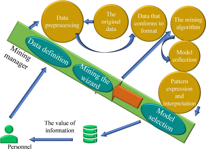
Data mining refers to the process of extracting meaningful information from large, incomplete, and noisy datasets17. With the rapid development of society and technology, data is now generated at an unprecedented rate, making it increasingly challenging to identify critical information within complex datasets18. As a method for managing, analyzing, and processing information, data mining plays a vital role in uncovering essential insights from massive amounts of data. The process typically involves filtering raw data to obtain relevant objects in a standardized format. These objects are then processed in the mining core to generate a set of patterns. Through further refinement, the system extracts valuable information, thereby completing the mining process19. The overall framework of the data mining process is illustrated in Fig. 1.

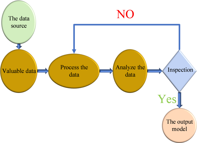
The specific steps of data mining vary across environments and can be adjusted to suit different contexts. These steps are fine-tuned depending on the scenario, as various data mining techniques possess distinct characteristics and operational processes. Figure 2 illustrates a generalized overview of the data mining process20.

Classification is a fundamental component of data mining and plays a central role in many mining systems21. It involves constructing a classification function based on training data and applying the model to categorize new, unprocessed data, enabling rapid and accurate predictions22. Commonly used classification algorithms include the following:
(1) Decision Tree Algorithm: This inductive algorithm constructs a decision tree model from a dataset, offering a straightforward and interpretable classification method23. It follows a top-down recursive approach: the root node is selected using attribute classification metrics, and the dataset is progressively partitioned into subsets. Each terminal leaf node corresponds to a category, and the paths from root to leaf define the classification rules. Figure 3 illustrates the principle of the decision tree algorithm, using gender characteristics as an example.

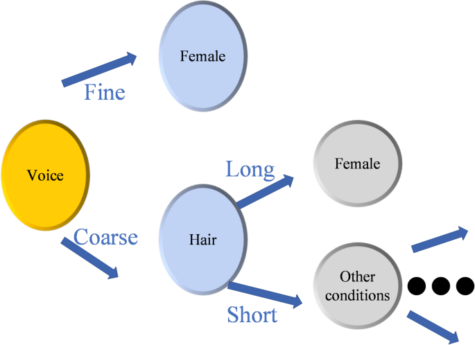
Principle flow of decision tree.
(2) Artificial Neural Network (ANN) Classification Algorithm: Based on the perceptron model, the ANN algorithm simulates the structure and function of biological neural networks. It is capable of automatic feature learning and requires minimal human intervention during the training and classification process24.
(3) Bayesian Classification Algorithm: This algorithm applies Bayes’ theorem to compute the posterior probability of an object based on its prior probability, assigning the object to the class with the highest posterior probability. Although similar in performance to decision trees and neural networks, the Naive Bayes classifier often demonstrates advantages in certain domains. A notable strength of Bayesian learning is its ability to update hypothesis probabilities incrementally with new training data, rather than discarding earlier hypotheses25. By combining prior knowledge, probabilistic reasoning, and observed data, Bayesian models not only make predictions but also quantify uncertainty—for example, estimating that “there is an 88% probability that the student will pass the exam” or “a 77% likelihood of rain tomorrow”26. However, Bayesian methods require prior knowledge of probability distributions, and computing the optimal hypothesis can be computationally expensive. In specific cases, this cost can be reduced. Figure 4 presents the principle of Bayesian classification with probability notations a and b.

(4) Support Vector Machine (SVM): The SVM is a widely used binary classification model27. Its core principle is to maximize the margin between data points in the feature space using a linear classifier28. For nonlinear classification tasks, SVM employs kernel functions to map the input data into a higher-dimensional space, where linear separation becomes possible. For linearly separable data, the dataset D can be represented as shown in Eq. (1):
$$D=\left\{ \left \right.\left),…\left. {({y_})} \right\}$$
(1)
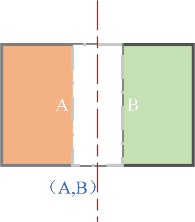
where Xi and Yi denote the feature vectors and category labels, respectively. Figure 5 illustrates the concept of a linearly separable dataset.

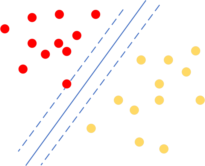
Linearly separable datasets.
As shown in Fig. 5, multiple lines or hyperplanes can separate the two data categories29. The key objective of SVM is to identify the optimal hyperplane that minimizes classification errors while maximizing the margin between the classes. The linear hyperplane can be expressed as shown in Eqs. (2),
$$\omega \cdot X+b=0$$
(2)
where ω represents the weight vector and b denotes the bias term. The margins H₁ and H₂ are defined in Eqs. (3) and (4).
$${H_1}:{\omega _0}+{\omega _1}{x_1}+{\omega _2}\times {}_{2} \geqslant 1,{y_i}=+1$$
(3)
$${H_1}:{\omega _0}+{\omega _1}{x_1}+{\omega _2}\times {}_{2} \leqslant – 1,{y_i}= – 1$$
(4)
The data points that lie directly on these margin boundaries are referred to as support vectors. Identifying the optimal hyperplane is formulated as a convex quadratic optimization problem, with the objective function defined in Eq. (5).
$$f=\hbox{min} \frac{1}{2}{\left\| {\left. \omega \right\|} \right.^2},{y_i}({\omega ^T}{x_i}+b),i=1…,n$$
(5)
The evaluation of classification performance relies heavily on the confusion matrix, which serves as a core tool in classification analysis. Figure 6 illustrates the detailed structure of the confusion matrix.

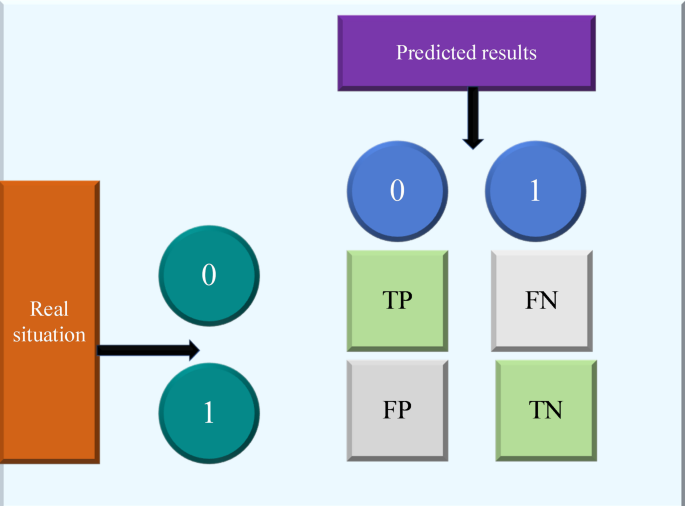
Figure 6 presents the four components of the confusion matrix, defined as follows:
True Positive (TP): A positive instance correctly classified as positive.
True Negative (TN): A negative instance correctly classified as negative30.
False Positive (FP): A negative instance incorrectly classified as positive.
False Negative (FN): A positive instance incorrectly classified as negative.
Based on these parameters, several evaluation metrics are derived to assess classification model performance:
Accuracy: Also referred to as the overall recognition rate, it measures the proportion of correctly classified instances across the entire dataset.
Precision: The proportion of correctly classified positive instances out of all instances predicted as positive, reflecting the reliability of positive predictions.
Recall: Also known as sensitivity, it measures the proportion of correctly identified positive instances, indicating the model’s ability to capture relevant cases31.
F1 Score: The harmonic mean of precision and recall, providing a balanced measure of a model’s classification performance. The F1 Score ranges from 0 to 1, with higher values representing better performance.
The formulas for these evaluation metrics are given in Eqs. (6)–(9).
$$accuracy{{=}}(TP+TN)/(P+N)$$
(6)
$$precision{{=}}TP/(TP+FP)$$
(7)
$$recall{{=}}TP/(TP+FN)$$
(8)
$${F_1}{{=}}\frac{{2 \times precision \times recall}}{{precision+recall}}$$
(9)
Ensemble learning algorithms are designed to combine the strengths of multiple models while compensating for their individual weaknesses32. In data mining, no single algorithm is without limitations, making ensemble methods particularly valuable. The central principle is to integrate diverse models in a manner that enhances the overall classification performance of the dataset33. Two widely used ensemble techniques are Bagging and Boosting.
Bagging (Bootstrap Aggregating): This method improves classification stability by combining the outputs of multiple base classifiers through majority voting. To reduce correlation among classifiers, Bagging generates diverse training datasets via resampling with replacement34. Each classifier then makes independent predictions, contributing to the robustness of the final model.
Boosting: This technique aims to improve classification accuracy by emphasizing the errors of prior classifiers. Base classifiers are trained sequentially, with each new model assigning greater weight to previously misclassified samples35. Through this iterative process, Boosting reduces misclassification rates and enhances overall performance36.
(1) In this study, several ensemble methods were applied. For example, RF, an implementation of Bagging, constructs multiple decision trees and aggregates their predictions through majority voting. The workflow of RF is illustrated in Fig. 7.

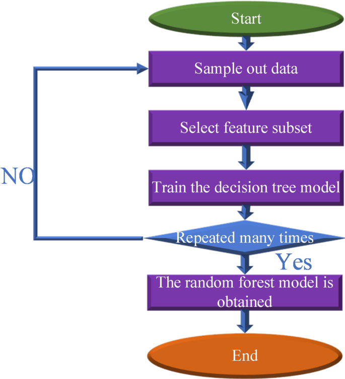
The classification performance of the RF algorithm largely depends on the quality of its individual decision trees37. When the decision trees perform well, the overall accuracy of the RF model improves. However, the effectiveness of RF decreases as the correlation between decision trees increases, since highly correlated trees are more likely to make similar errors38. The degree of correlation is influenced by the number of features selected (denoted as m). A larger m generally results in stronger correlations among trees. To address this, the RF algorithm employs the bootstrap sampling method. Samples excluded during the bootstrap process, known as out-of-bag (OOB) samples, are used to estimate the model’s error rate. The calculation of the OOB error rate follows three steps: (1) Each OOB sample is classified using the RF model. (2) The final classification is determined by aggregating the votes from all decision trees. (3) The OOB error rate is computed as the ratio of misclassified OOB samples to the total number of samples. This error rate provides an unbiased estimate of the RF model’s generalization performance39.
Model building based on GA
Current approaches to mental health education for sports education students lack sufficient personalization and adaptability. As a result, the identification of mental health issues is often delayed and ineffective, negatively affecting students’ learning and daily lives. To address this gap, this study integrates big data and IoT technologies to develop an adaptive mental state perception model aimed at providing accurate and timely mental health support, thereby improving students’ psychological well-being. The problem is defined as follows: how can mental health education pathways be optimized using big data and IoT technologies to enhance mental state recognition and intervention? The study’s objectives are to mine and analyze student mental state data, then construct and refine a model capable of effectively perceiving mental states. The methodology involves four main steps: data collection and preprocessing, algorithm selection and optimization, model training, and performance evaluation. Initial analyses employ basic classification algorithms, including decision trees, SVM, and RF. Subsequently, a GA is introduced to optimize feature selection, leading to the development of a GA-RF mental state perception model. In this framework, GA is used to refine input features, reduce redundancy, and improve training efficiency, thereby enhancing classification accuracy. The optimized features are then used to train the RF model, which is further improved with GA integration to form the GA-RF model. The model’s performance is evaluated using standard metrics such as accuracy, recall, and F1 score. These steps highlight the systematic and effective nature of the approach, providing strong support for mental health education in sports education.
Input optimization serves two main purposes: Model Performance Enhancement: Network behavior records can involve multiple dimensions, often with low information density. Even after preprocessing, as many as 50 dimensions may remain. Using all of them for model training can significantly slow computation and reduce predictive accuracy due to redundant or irrelevant features. Feature selection compresses the dimensionality of the data, shortening training time and improving classification accuracy by eliminating extraneous inputs. Data Storage Optimization: As the data volume increases, so does its dimensionality, which directly expands the storage scale. Input optimization through dimensionality reduction reduces storage costs and makes large datasets easier to manage efficiently and economically.
In selecting classification algorithms for psychological state perception, this study considered several widely used methods, including Decision Tree, SVM, RF, and ANN. Each of these algorithms has demonstrated strong performance across various classification tasks. However, this study placed particular emphasis on algorithm performance in high-dimensional settings, feature selection, and model stability. Based on these criteria, the GA-RF model was chosen. RF, an ensemble learning algorithm based on the Bagging strategy, classifies data by training multiple decision trees and aggregating their outputs through a voting mechanism. It is well-suited for handling high-dimensional and nonlinear data, as well as noisy and imbalanced datasets. These strengths are particularly important in psychological health analysis, where network behavior features often exhibit noise and complex nonlinear relationships. Moreover, RF effectively reduces overfitting and improves model generalization. The integration of GA primarily serves to optimize feature selection. Psychological health network behavior datasets typically contain numerous features with considerable redundancy, which can reduce both the efficiency and accuracy of direct classification. GA, by simulating the process of natural selection, identifies optimal feature subsets, thereby reducing dimensionality and enhancing prediction performance. This feature selection process not only improves RF’s classification effectiveness but also accelerates model training. Compared with standalone RF or other classification algorithms, the GA-RF model combines GA’s optimization capabilities with RF’s ability to process high-dimensional data, resulting in superior performance in psychological state perception tasks. Experimental results demonstrated that the GA-RF model outperformed comparison algorithms such as SVM and Decision Tree in both accuracy and F1 score for depression classification, further validating its practical value in psychological health education.
In summary, the GA-RF model was selected because of its ability to effectively manage high-dimensional, nonlinear, and noisy data while enhancing classification performance through GA-optimized feature selection. This combined approach improves computational efficiency without compromising accuracy, offering stable and reliable results. Accordingly, the GA-RF model represents the optimal solution for psychological state perception in sports education.
GA was employed for input optimization in the algorithmic framework to identify the most informative feature subsets from large datasets. This process involved selecting the best feature combinations across multiple dimensions. The feature selection procedure using GA is outlined as follows:
GA, inspired by Darwin’s theory of evolution, operates on the principle of natural selection to identify optimal solutions. In feature selection, GA employs a binary encoding scheme in which each bit corresponds to a feature in the vector. A bit value of “1” indicates that the feature is selected, while a value of “0” denotes its exclusion. The features encoded as “1” are then used to construct the classifier. The core of GA’s training process lies in iterative operations on sample data, guided by fitness function values and selection strategies, to identify the optimal feature subset. Wu et al.40 demonstrated that technology-driven teaching methods significantly enhance student development, thereby supporting the effectiveness and feasibility of this approach for exploring adaptive mental health pathways in sports education.
In this study, the genetic optimization algorithm adopts a distance-based criterion for the fitness function, simplifying analysis by directly evaluating sample information. It measures sample validity by analyzing the distances between similar and dissimilar samples. The specific computational methods are given in Eqs. (10) and (11). The within-class scatter matrix Sw is defined in Eq. (10):
$$\begin{gathered} {S_w}=\sum\limits_{{i=1}}^{c} {P({\omega _i})E\{ (X – {M_i})(X – M_{i}^{T})\} } \\ =\sum\nolimits_{{i=1}}^{c} {P({\omega _i})\frac{1}{{{N_i}}}\sum\nolimits_{{k=1}}^{{{N_i}}} {(X_{k}^{i} – {M_i})(X_{k}^{i}} – {M_i}{)^T}} \\ \end{gathered}$$
(10)
Overall interclass scatter matrix Sb can be expressed as shown in Eq. (11):
$${S_b}=\sum\nolimits_{{i=1}}^{c} {(P({\omega _i})E} \{ ({M_i} – {M_0}){({M_i} – {M_0})^T}\}$$
(11)
\(P({\omega _i})\)refers to the prior probability of a class, which is based on the criterion fitness function of distance. When the intra-class sample distances decrease and the inter-class sample distances increase, the classification quality of the corresponding model improves, as expressed in Eq. (13).
$$J=\frac{{tr({S_b})}}{{tr({{\text{S}}_{\text{w}}})}}$$
(12)
In Eq. (13), c denotes the number of categories, determined according to the distance-based fitness function. \(P({\omega _i})\) represents the prior probability of each class. Mi and M correspond to the mean vector of the i-th class and the mean vector of the overall sample set, respectively. Their values are defined in Eqs. (14) and (15).
$${M_i}{\text{=}}\frac{1}{{{N_i}}}\sum\nolimits_{{k=1}}^{{{N_i}}} {X_{k}^{i}}$$
(13)
$$M=\frac{1}{N}\sum\nolimits_{{i=1}}^{N} {{X_i}=} \sum\nolimits_{{i=1}}^{c} {P({\omega _i}){M_i}}$$
(14)
The GA employs a random sampling method with replacement to select individuals based on their fitness values. Individuals with higher fitness scores have a greater probability of being retained for the next generation. This selection probability is expressed in Eq. (15).
$${P_i}=\frac{{\sum\nolimits_{1}^{i} {{J_i}} }}{{\sum\nolimits_{{i=1}}^{N} {{J_i}} }}$$
(15)
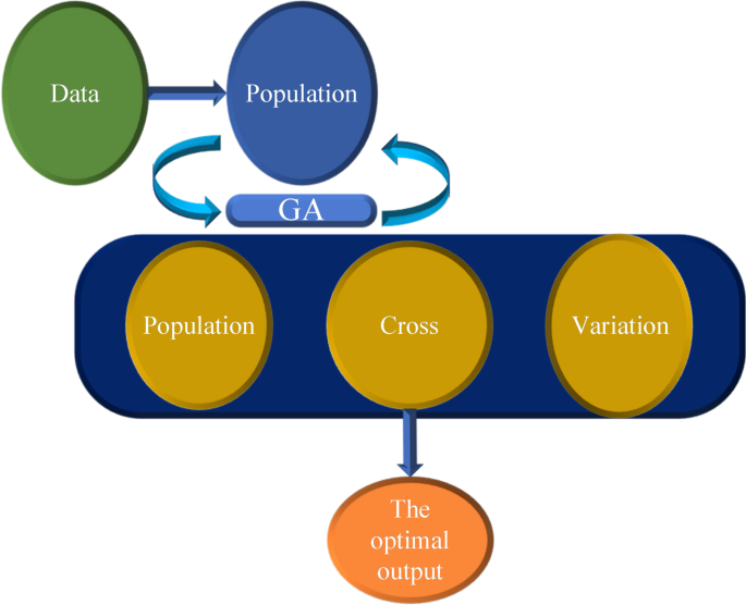
Figure 8 illustrates the detailed training workflow of the GA.

The workflow of the GA-RF mental health perception system developed in this study is illustrated in Fig. 9, covering the full closed-loop process from data collection to decision support. Initially, IoT devices deployed across the campus continuously collect multidimensional behavioral data from sports education students, including learning duration, exercise frequency, and social activity levels. The raw data are first processed through a preprocessing module to remove noise and fill in missing values, after which feature engineering generates derived indicators. Next, the GA performs an adaptive search across the high-dimensional feature space. Through iterative selection, crossover, and mutation operations, the algorithm identifies the most discriminative subset of features. This optimized feature subset is then fed into the RF model for training. By aggregating the predictions of multiple decision trees through a voting mechanism, the model outputs classifications of students’ psychological states. Finally, the predicted mental health indicators, such as depressive tendencies, trigger the teaching management system to generate personalized intervention strategies, such as adjusting training schedules or initiating psychological counseling. This creates an adaptive education pathway following the “perception–prediction–intervention” cycle. The collaborative optimization of the GA and RF is central to this architecture, effectively addressing high-dimensional feature redundancy while ensuring stable and accurate classification.

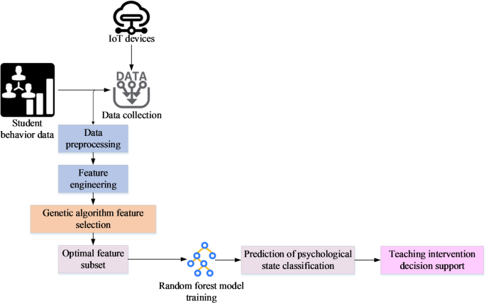
Workflow architecture of the GA-RF mental health perception system.
Following these steps, GA is applied to construct the perceptual model using network behavior data. The optimized feature subset identified by GA is then used to train the RF model, resulting in the GA-RF mental state perception model. Subsequently, the performance of four models—Decision Tree, SVM, RF, and GA-RF—is evaluated and compared. Notably, Li et al. (2019)41 demonstrated an interaction between social personality and online privacy, highlighting a causal relationship that is relevant to the context of this study.
Simulation experiment
Currently, the psychological health of students majoring in sports education has garnered significant attention from both educational institutions and government agencies. Influenced by multiple factors, these students are at risk of developing abnormal psychological conditions, which can lead to various negative outcomes. The dataset used in this study was obtained from the log servers and campus IoT data platform of a sports university. It includes students’ course learning records, athletic training data, and select daily life behavior data. All data were anonymized during collection to ensure the protection of personal privacy. The data collection process complied with ethical approval procedures, and all participants provided informed consent. Prior to model input, the raw data underwent rigorous preprocessing. Missing values were imputed, and noisy data were smoothed or removed. Features across different dimensions were standardized to ensure consistency in measurement scales. Additionally, expert annotations and questionnaire assessments were used to classify samples according to students’ psychological states, resulting in a high-quality training dataset. The initial dataset exhibited class imbalance, particularly with a lower proportion of samples showing depressive tendencies. To address this, a combination of SMOTE (Synthetic Minority Over-sampling Technique) and undersampling was applied, ensuring a more balanced distribution of classes within the training set and reducing classification bias. A total of 1,220 samples were included in the experiment. Each student’s identity was anonymized, with unique serial numbers used for identification. Behavioral features linked to these serial numbers constituted the dataset for comparative analysis. The study evaluated the performance of classification models in detecting internal and external tendencies, as well as a depression dichotomy model, providing a basis for understanding and improving psychological health assessment in sports education students.
The 1,220 samples used in this study were obtained from the IoT log databases of three institutions: East China University of Science and Technology, Hebei Sport University, and Chengdu Sport University, covering three major geographic regions: the eastern coastal area, the North China Plain, and the Southwest Basin. The sample population included undergraduate students in sports education and graduate students in athletic training, with a male-to-female ratio of 1.3:1 and an age range of 18–25 years. Data collection spanned two full academic years and covered typical scenarios such as regular teaching periods, final examination weeks, and provincial-level competition training sessions, effectively capturing multiple psychological stressors, including academic pressure and competition anxiety. The raw dataset included 50 features representing learning behaviors, training intensity, social activity frequency, and daily routines. K-means clustering confirmed the presence of four balanced behavioral patterns. Although the sample size was constrained by institutional data access policies, the multi-region, multi-scenario coverage partially mitigates biases from a single institution, providing a foundation for model generalization. Future work aims to expand dataset diversity by incorporating data from western vocational sports institutions through a university–industry collaboration framework. To enhance model generalization under the current dataset limitations, three methodological strategies were employed. First, transfer learning was applied: the GA-RF model trained on source institutions is adapted to target institutions, requiring only a small number of new samples for fine-tuning. Second, a dynamic feature importance monitoring mechanism was implemented. This mechanism detects shifts in the relationship between behavioral features and psychological states when the model is deployed in new environments, and it automatically triggers recalibration. Third, a synthetic data generation module was developed. It uses conditional generative adversarial networks to simulate behavioral patterns from different institutions, thereby increasing the diversity of training samples.
In terms of model selection, traditional classification algorithms such as Decision Tree, SVM, and RF were initially compared. Considering the characteristics of high-dimensional, noisy data, RF was selected as the base classifier, and GA was applied for feature selection and parameter optimization. Key model parameters included the number of decision trees and maximum depth in RF, as well as the number of iterations and population size in GA. Cross-validation combined with grid search was used to fine-tune these parameters, ensuring robust generalization across different dataset scales. The GA-RF fusion model was chosen based on three key characteristics of sports student behavioral data: high dimensionality, strong noise, and nonlinear associations. Compared with SVM, whose computational complexity increases sharply in high-dimensional settings, RF’s feature subsampling and ensemble mechanism provide inherent noise robustness. Compared with neural networks, which require large datasets, RF performs more reliably on small-scale educational data. The introduction of GA addresses feature redundancy: traditional filter-based feature selection methods often ignore feature interactions, whereas GA adaptively searches for optimal feature subsets through population evolution. Its crossover and mutation operations preserve complementary feature combinations. Parameter configurations were optimized based on the characteristics of educational data. For the RF model, 200 trees were used to balance accuracy and efficiency, and the maximum depth was set to 10 to prevent overfitting. The GA was configured with a population size of 50, 100 iterations, a crossover probability of 0.8, and a mutation probability of 0.01 to ensure thorough exploration of the feature space. Hyperparameter optimization was performed using grid search. For GA selection strategies, both roulette wheel and tournament selection were tested, with tournament selection ultimately chosen to improve convergence efficiency. For RF splitting criteria, Gini impurity and information gain were compared, and Gini impurity was selected for faster computation. All parameters were iteratively fine-tuned on the validation set to ensure model generalizability.
To evaluate the model’s performance across datasets of varying sizes, the experiment was divided into three groups: (1) a small-scale dataset with 1220 samples, (2) a medium-scale dataset with 2500 samples, and (3) a large-scale dataset with 5000 samples. Each dataset group was analyzed using the same set of algorithms, including Decision Tree, SVM, RF, and GA-RF.
link